Amateur Radio Astronomy
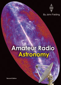
For everyone interested in radio astronomy Amateur Radio Astronomy is a great source of material to expand your knowledge and also provides a practical guide to making and setting up your own equipment, through to the study signals coming from space.
Click cover picture to buy this online.
Corrections, updates and additional information
Corrections to Chapter 1
Page 25
Construction was started in the spring of 1952 and was expected to take 3 years, but was only eventually completed in late 1957 after many dramas over the escalating cost, design problems, and supply of steel and changing requirements as the new science evolved. It was named The Nuffield Telescope or Jodrell Bank MK1, a 250-foot parabola the largest of its type in the world at that time. The full account of this and subsequent developments are covered in Lovell’s books, The Story of Jodrell Bank, Out of the Zenith and Astronomer by Chance.
Corrections to Chapter 4
Page 111
Antenna gain is also in direct proportion to the effective aperture size (capture area) of the antenna. It is relatively easy to see the connection between the physical size of a parabolic dish or dipole array and the apparent gain, but in the case of a Yagi or other types of antenna, it is not so obvious.
Page 112
Antenna Effective Aperture Equation
The effective aperture (capture area) of a parabolic antenna is expressed in terms of the area, Aphys, by:
Ae = Aphys x h
Where:
Ae is the effective aperture area, m2
h is the aperture efficiency.
Aphys is the actual collecting area of the antenna, m2.
Page 116
Below is listed some experimental data obtained from various Yagi antennas obtained by Fishenden and Wiblin.
|
No of Directors |
Beamwidth, |
Gain over |
Gain per element |
|
30 |
22 |
||
|
20 |
26 |
21 |
0.95 |
|
13 |
31 |
15 |
1.00 |
|
9 |
37 |
13 |
1.18 |
|
4 |
46 |
8 |
1.33 |
Note: The beamwidth in the above table are measured at the –6dB points and not the more normal –3dB points.
Correction to Chapter 6
Pages 180-181
A complication is that the Earth is inclined on its axis by an angle of approx. 23.5°. This can be shown by redrawing the celestial co-ordinates as illustrated below in Figure 6.2. From this can be drawn the “ecliptic plane” which is the apparent path traced by the Sun as the Earth rotates during a sidereal day. From this can be seen the derivation of the point on the celestial equator known as the “vernal equinox”, commonly known as the “First point of Aries”, this is the point where the ecliptic plane and the celestial equator intersect. (On Earth this is similar to the zero degree longitude reference point taken as being Greenwich).
A measurement made from the vernal equinox point on the celestial equator eastwards is called Right Ascension; this is conventionally expressed in hours and minutes. On Earth the other coordinate is the latitude, measured along another meridian as degrees north or south of the equator. The equivalent measurement on the celestial sphere is Declination, measured again in degrees along another meridian north or south of the celestial equator. It is the convention to use + for objects North and – for objects South of the equator.
Right Ascension can also be expressed in degrees. Because the Earth takes 24 hours to complete one rotation one hour is equivalent to 15°. So, for example, a right ascension of 36° could be expressed as 1/10 of a day, i.e. 2.4 hours or a right ascension of 2hr 24minutes. Note that RA is always measured eastwards along the celestial equator from the vernal equinox reference point.
Converting from the RA and Declination to azimuth and elevation for a particular location can be done using standard formula but a much simpler method is to utilise one of the many software packages available at low cost. The writer uses a package called “Radio-Eyes” written by Jim Sky. This software gives a view of the sky from the observer’s location and converts the RA and Dec of an object to antenna azimuth and elevation. (Because the view is looking down from space to the observer’s location the azimuth is reversed to the normal. If you imagine looking up from the observer’s point the azimuth is then correct).
When an objects apparent position in the sky is given in astronomical tables it is important to state the exact date and time this was established, this is called the “epoch”. Hence, this epoch time is always appended to the data.
For example, Vega would be given as “5hr 24m, 38° 45’N (1950.00)”. This means the exact time was 00h 00m on the 1st of January 1950, or it has been corrected back to that time.
(The alternative way of writing this would be “5hr 24m, +38° 45’ (1950), because the declination is North and the 1950 assumes the first minute of 1st January 1950).
Corrections to Chapter 9
Page 236
The temperature of the two sources needs to be known accurately, TH and TC being the hot and cold sources in degrees Kelvin. Knowing the two source temperatures and the Y factor the noise factor (F) can be calculated using the formulas. Noise Figure is the logarithm of the noise factor.
TH –Y
Te = ¾¾¾¾¾
Y – 1
Te
F = ¾¾¾ + 1
290
Rear Cover
4120MHz should read 1420Mhz.
Category: Books Extra